Introduction
I often feel when talking to coworkers, practitioners and people in general that the Bayesian philosophy has to prove it’s worth or justification as if it’s a contender to the existing way. In reality, of course, the more prevalent way of working with probabilities is a specialization of the Bayesian formalism. Not the other way around. As such, I often find myself wondering why this came to be. Truth be told, I think the majority of the scientific community just forgot the reason for working with pure maximum likelihood. It’s a good reason, and was on top of that necessary to make any kind of progress on interesting problems at the time. The mathematical tooling as well as the computational power has increased dramatically since the introduction of pure maximum likelihood, and the reason for using it basically no longer exist. So, in this post I hope to get you more familiar with the Bayesian way of thinking and hopefully also showing you that it’s not really that scary at all. Specifically, this post will be dedicated to show you for a couple of model how the results are affected by your prior assumptions as well as the size of your data.
Let’s start off with the basics. In general throughout this post I will refer to the prior \(p(\theta)\), likelihood \(p(y | \theta)\) and posterior \(p(\theta | y)\). We will be looking into a convenient Bayesian model called the Beta binomial model which is useful for modeling a discrete number of positive outcomes out of \(N\) binary trials. This features a Beta prior distribution. We’ll further work with the assumption that we’re modeling the number of Startups that made it to Unicorns, i.e., they’re worth a billion dollars.
Starting the modeling exercise
In the example outlined we’re modeling the number of companies who made it to Unicorns, and we gathered a list of \(N=10\) companies and checked how many of them are unicorns. In this case we got 3 unicorns and 7 “normal” companies. Let’s set up a model for this now. We will denote the number unicorns by \(y\sim~Bin(N, \theta)\) where N is the number of companies in the survey and \(\theta\) is the unknown probability of a company becoming a unicorn. The prior is given by the beta distribution \(\theta\sim B(\alpha, \beta)\). This particular setup has a closed form solution which allows us to directly infer the posterior distribution of our parameter \(\theta\).
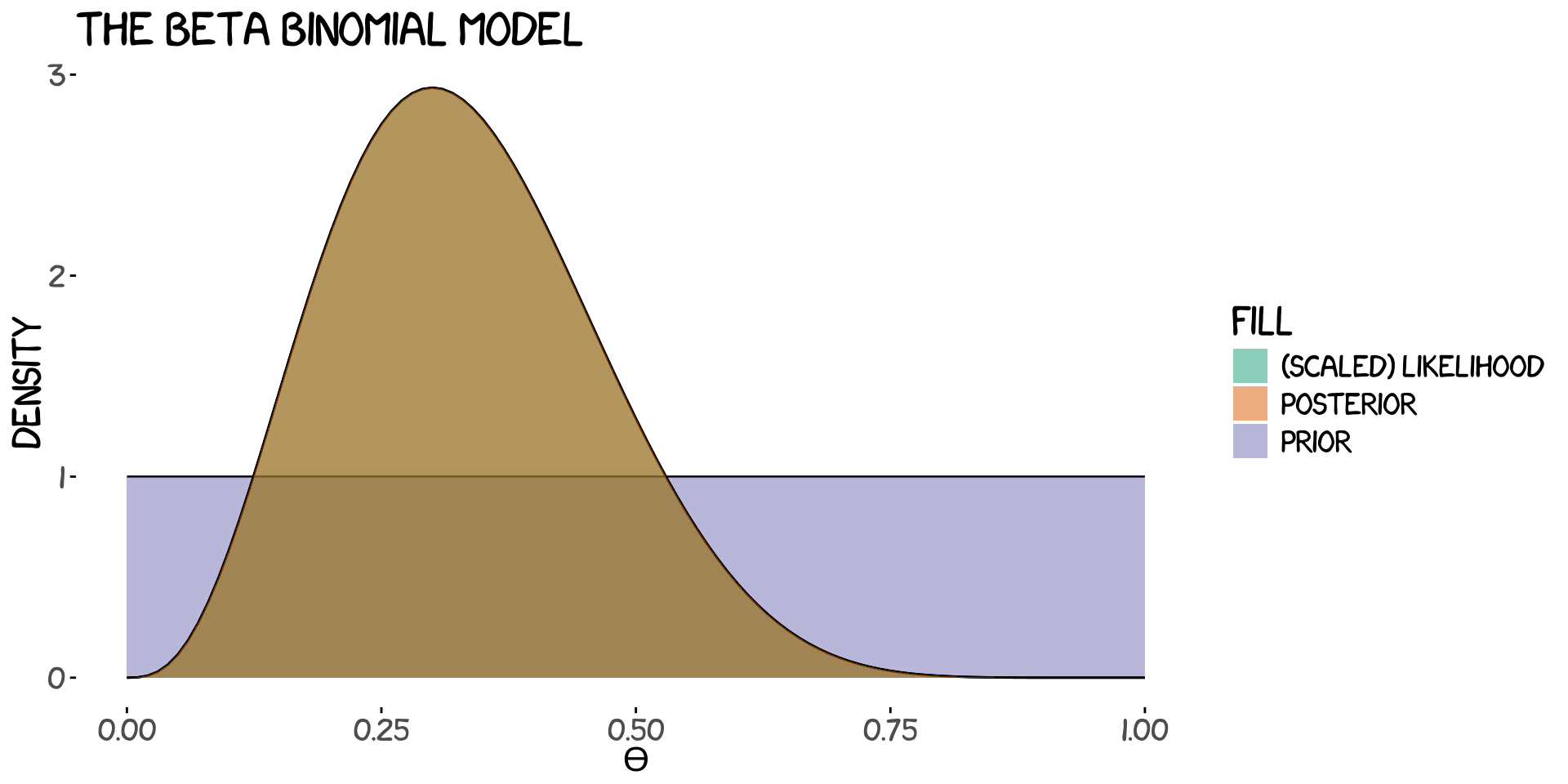
Before inferring the posterior we need to choose values for our prior. In this case, \(\alpha\) and \(\beta\). There are a number of ways to do this, and depending on who you are and what you believe they will differ. Believe me when I say that this is a good thing. I’ll begin by showing you what would happen if we claim complete ignorence which would correspond to a flat prior which in Beta distribution language is \(\alpha=1\), \(\beta=1\). Our prior, likelihood and posterior look like this.

Ehhh, wait a minute.. Where’s the posterior and likelihood? Well, remember that we said we were completely ignorant right? Right, so that would correspond to trusting the data blindly and just accepting that we have no knowledge to add. So we end up with the following results
| Estimate | α | β | Average | NA |
|---|---|---|---|---|
| prior | 1 | 1 | 0.5000000 | 0.2886751 |
| posterior | 4 | 8 | 0.3333333 | 0.1307441 |
which states unsurprisingly that the probability for a company to become a unicorn is 33%. Well, that’s total BS. We trusted the data without accounting for all the biases that happens to us when we collect or think about data. In this very example here we only have 10 companies and we just picked companies we’ve heard of many times which increases the possibility of them being unicorns.
A better prior gives a better model
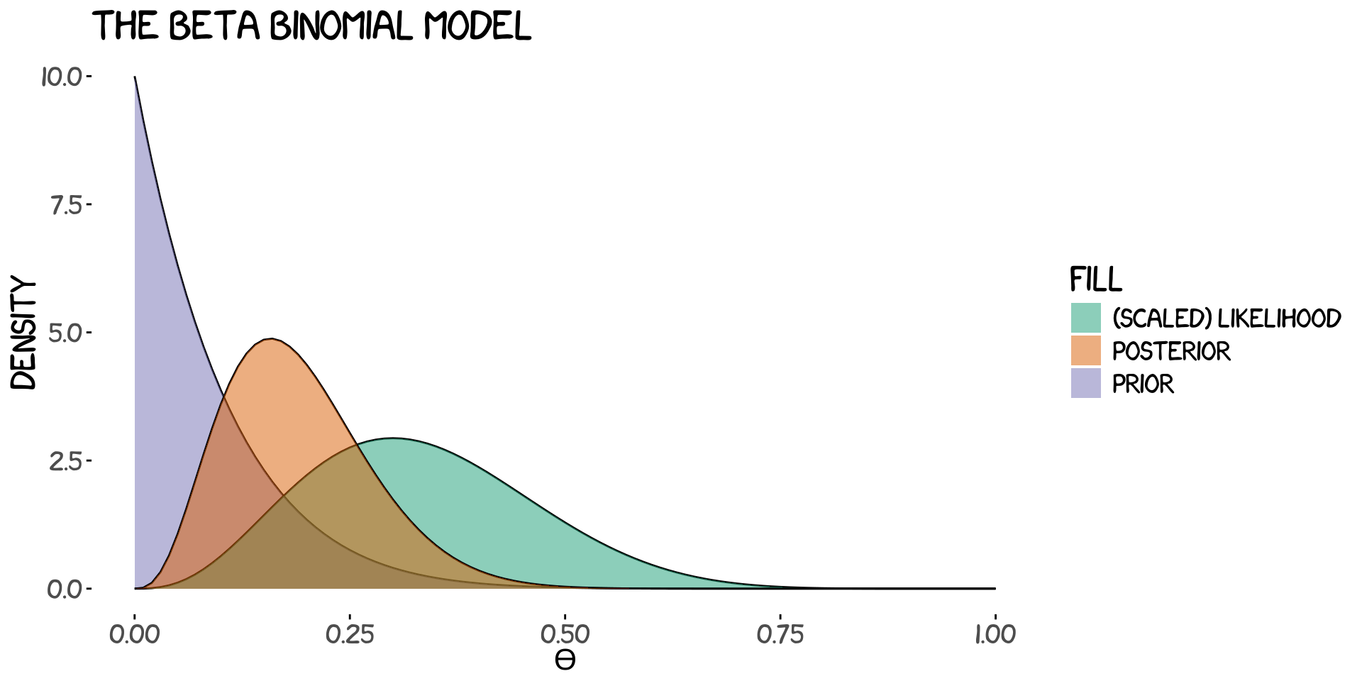
Let’s try again but this time let’s pretend that we’re not vegetables and actually have some idea about how many companies actaully make it to unicorn level. I would say in general that chances are slim so I will choose a prior distribution that reflects that belief. In this case I’m going with \(\alpha=1\), \(\beta=10\). We can see the immediate results below in the plot and the table.

Now it’s abundantly clear that I don’t believe it’s very probable for a given company to become a unicorn. In fact we’re shy of a posterior average change of 20%.
| Estimate | α | β | Average | NA |
|---|---|---|---|---|
| prior | 1 | 10 | 0.0909091 | 0.0829883 |
| posterior | 4 | 17 | 0.1904762 | 0.0837190 |
As a small eye-candy I’ve animated the process where we change the prior assumption from uninformed to informed and how the data interacts with it to create the posterior.

Summary
In this post we went through a few scenarios and consequences of choices for our model. It’s important to note that the process here is not something I would recommend. The prior should never be adapted to fit your data. It should be a reflection of your knowledge. I basically just wanted to show you what happens when you don’t add your knowledge to your models, as well as highlighting the dangers of maximum likelihood.
Credits
Ideas for the plots and the Beta binomial model was shamelessly stolen from The Bayes rules! book. Check it out!