Introduction
I have been working with neural networks for the better part of 25 years, and for most of the last seven or eight of those, transformers have been the air everyone breathes. I use them, I fine-tune them, and I have a strong opinion about why we should be careful about building everything on a foundation controlled by three labs on another continent.
Sitting in the summer house in Sweden I had the time to re-read “Attention Is All You Need” (Vaswani et al. 2017). And as usual nodded along, filed the architecture diagram somewhere in the back of my head, and moved on. After a couple of days I wondered why I could not intuitevely account for why each piece is there, in the order it’s there, without reaching for the paper again.
So I did the thing I always do when I want to understand something. I tried to rebuild the transformer from the bottom up, starting from the simplest possible version of “attention” and only adding a piece when it solves a problem.
This post is the writeup. It’s a technical deep dive, with the same spirit as the JEPA one. By the end we’ll have a single transformer block in Julia, every line of which I can justify from a problem I hit on the way there. The architecture itself is really a series of very sensible answers to very specific questions, and once you’ve asked the questions yourself the answers stop feeling like magic.
The problem with reading left to right
You have a sequence. A sentence, a time series, a string of tokens. You want to produce a representation of each position that knows about the rest of the sequence, because the meaning of “bank” depends on whether “river” or “investment” is nearby, and the meaning of a price tick depends on what the market has been doing all morning.
For a long time the answer was the recurrent neural network (RNN). Read the sequence left to right, one token at a time, carry a hidden state forward, and let each step’s representation be a function of the hidden state, which is a function of the hidden state before it, all the way back to the start. It kinda works. But, two things go wrong with that. First, information from the start of the sequence has to survive a chain of matrix multiplications to reach the end, and the chain is unkind. Gradients either vanish or explode, and even when they behave, the model has to learn to copy the relevant bit forward through every intermediate step. Second, and more prosaically, you cannot parallelise it. Token fifty cannot be computed until token forty-nine is done. On modern hardware that’s a minor inefficiency that becomes the reason a training run takes a month instead of a weekend.
So let’s ask a question. What if we just let every token look at every other token, all at once?
The first move: everyone looks at everyone
For each token in the sequence, build its new representation as a weighted average of all the tokens, including itself. If “bank” should care more about “river” than about “the”, let the weight on “river” be larger.
That’s the whole first move. A weighted average, computed for every position, in parallel. Right away you have to decide the weights. You could hand-craft them (a window around the word, say), but that throws away the point, which is that relevance is context-dependent and the model should learn it. So the weights have to be a function of the tokens themselves.
The cheapest possible notion of “token \(i\) is relevant to token \(j\)” is: do their embeddings point in a similar direction? A dot product answers exactly that. So let the weight from \(i\) to \(j\) be the dot product of their embeddings, \(x_i \cdot x_j\). Stack every pair into a matrix and you get \(X X^\top\), which is \(n \times n\), i.e., every token against every token, all at once, on the GPU, exactly the thing where RNN struggles. That’s the unnormalised self-attention matrix.
The output for each token is a weighted sum of everyone’s embeddings, weighted by those similarities. In matrix form that’s the attention matrix times the embeddings.
\[\text{out} = (X X^\top)\, X\]
And you’re done. That’s self-attention in its rawest form, no learned weights anywhere in it. The embedding of each token plays every role at once: it’s the thing you compare for similarity, and it’s the content you average in. One vector, two jobs. We won’t dive into embeddings in this post as that is worth it’s own seperate post.
Softmax, and the scaling that saves the day.
The raw \(X X^\top\) is a disaster as a set of weights, because dot products are unbounded. A token that happens to have large entries gets a huge weight, swamps the average, and the whole thing degenerates. We want weights that sum to one across each row, so each output is a proper convex combination. That’s softmax, applied row-wise.
\[\text{out} = \text{softmax}(X X^\top)\, X\]
However, if your feature dimension \(d\) is large, the dot products \(x_i \cdot x_j\) grow like \(\sqrt{d}\) in expectation (they’re sums of \(d\) zero-mean terms), and their variance grows like \(d\). Push a vector with entries of size \(\sqrt{d}\) through a softmax and you get something close to a one-hot which is hardly what we want because the gradients through the softmax go flat. The model learns nothing, because the softmax is saturated.
The fix is to divide the logits by \(\sqrt{d}\) before the softmax.
\[\text{self\_attention}(X) = \text{softmax}\!\left(\frac{X X^\top}{\sqrt{d}}\right) X\]
It’s easy to underestimate that \(\sqrt{d}\) term since it’s just “a scaling factor”. But, take it out and your large-model training silently stalls. The scaling is what keeps the logits in the regime where softmax actually has a usable gradient. The whole thing can be expressed easily in Julia.
function self_attention(X)
    d = size(X, 2)                    # feature dimension, read off the input
    scores = X * X' / sqrt(d)        # (n, n) similarity logits
    weights = softmax(scores; dims=2)
    return weights * X               # (n, d)
end
Six lines, and it’s the entire mechanism. Everything else in a transformer is plumbing so you can stack this on top of itself.
A worked example: an apple and a banana
Formulas are one thing. Let me run the six lines by hand on a sentence so you can watch the numbers move.
The sentence is “an apple and a banana” (five tokens). I’m going to use a feature dimension of three, and I’m going to name them tech, fruit, grammar. Each token starts life as a little 3-vector saying how much it carries of each. Here are the starting embeddings, the \(X\) matrix.
| token | tech | fruit | grammar |
|---|---|---|---|
| An | 0.0 | 0.0 | 1.0 |
| apple | 0.7 | 0.8 | 0.0 |
| and | 0.0 | 0.0 | 0.5 |
| a | 0.0 | 0.0 | 1.0 |
| banana | 0.0 | 0.8 | 0.0 |
The two determiners are pure grammar. The conjunction is half-strength grammar. The interesting ones are apple and banana. apple is polysemous, i.e., it carries both tech (Apple the company) and fruit (apple the fruit), and I’ve made it fruit-heavy by a hair. banana is unambiguously fruit only, no tech. In the context “an apple and a banana” the fruit reading is the one a human picks for both, and the question is whether one pass of attention can use banana’s unambiguous fruit to pull apple away from tech and toward fruit.
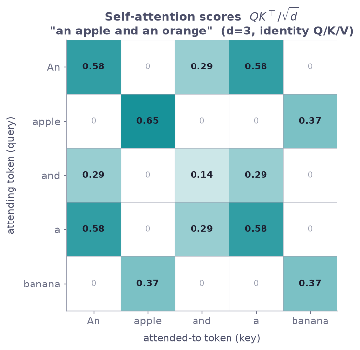
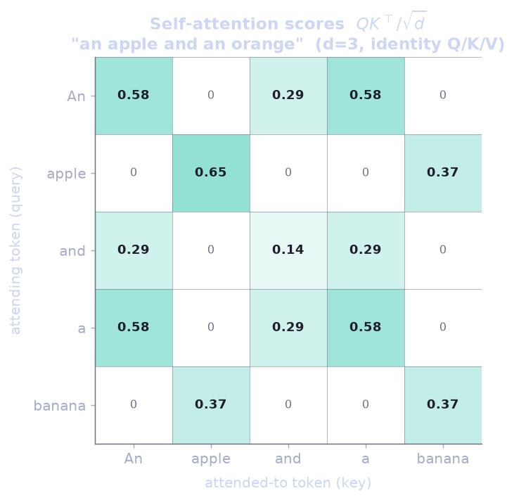
Now lets apply self-attention from the last section, with no learned weights. the score between two tokens is just their dot product, which is their cosine similarity times their magnitudes. Tokens that look alike attend to each other. The score matrix \(X X^\top/\sqrt{d}\) becomes:
| An | apple | and | a | banana | |
|---|---|---|---|---|---|
| An | 0.58 | 0 | 0.29 | 0.58 | 0 |
| apple | 0 | 0.65 | 0 | 0 | 0.37 |
| and | 0.29 | 0 | 0.14 | 0.29 | 0 |
| a | 0.58 | 0 | 0.29 | 0.58 | 0 |
| banana | 0 | 0.37 | 0 | 0 | 0.37 |
Look at the structure before we even softmax. The matrix is blocky. apple and banana only see each other (and themselves). The three grammar tokens (An, and, a) only see each other. The sentence has fallen into two clusters, the two nouns and the three function words, purely from dot-product similarity. That’s the parallel structure of “an X and a Y” showing up as a pattern in the numbers, with no rule telling the model it’s a list.
(Aside: with \(d=3\) the \(\sqrt{d}\) scaling barely moves the logits, which is why I said earlier it’s a large-\(d\) fix. Squash these by 1.73 and the softmax is still well-behaved. Do the same at \(d=4096\) without the scaling and the softmax turns to one-hot. Same math, different regime.)
Now softmax each row and multiply by \(X\) again to get the new embeddings. Let me do apple in full, because it’s the interesting one. Its row of logits is \([0,\, 0.65,\, 0,\, 0,\, 0.37]\). Softmax turns that into weights over \([\text{An, apple, and, a, banana}]\).
\[w_{\text{apple} \to \cdot} = [0.16,\, 0.30,\, 0.16,\, 0.16,\, 0.23]\]
So apple attends to itself at 0.30, to banana at 0.23, and splits the remaining 0.47 evenly across the three grammar tokens it has zero similarity with (they get the softmax floor, the uniform weight that keeps the row summing to one). The new apple embedding is that weighted average of the values below.
\[\text{apple}_{\text{new}} = 0.16\,\text{An} + 0.30\,\text{apple} + 0.16\,\text{and} + 0.16\,\text{a} + 0.23\,\text{banana}\]
Crunch the numbers and:
| token | before | after |
|---|---|---|
| apple | [0.70, 0.80, 0.00] | [0.21, 0.42, 0.39] |
| banana | [0.00, 0.80, 0.00] | [0.17, 0.39, 0.42] |
| An | [0.00, 0.00, 1.00] | [0.10, 0.23, 0.61] |
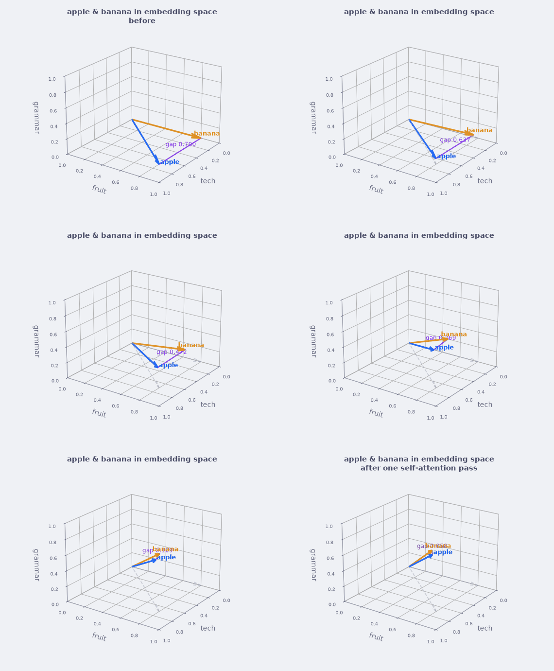
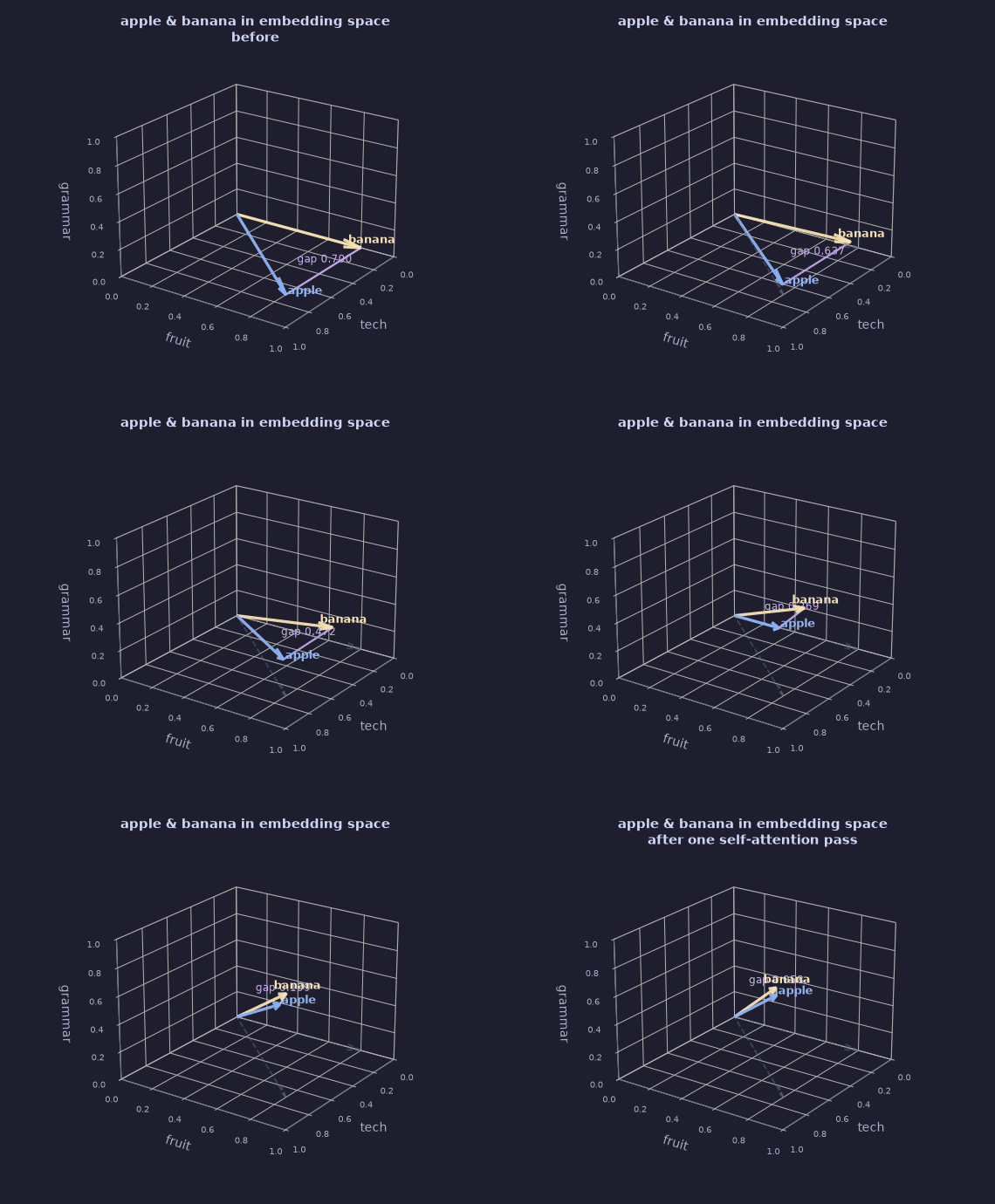
Here are the two nouns as actual vectors in the tech/fruit/grammar space. The dashed ghosts are their starting positions; the solid arrows are where one pass of self-attention lands them. They swing up into grammar (pulled from the determiners) and close to within a twelfth of their starting distance, the gap dropping from 0.700 to 0.059. Thus, attention pulls similar vectors toward each other.
For the keen observer you will see a bubu here since I made this heatmap before I wrote the text and I use Q,K, V notation where Q=XW with W=I. When writing the post I thought it was better to start with the raw embeddings. So yeah. In the plot above there is only X.
Now regarding the plot three things happened here. First, information moved. The nouns pulled grammar up from zero to 0.37, straight out of the determiners. The determiners pulled a little tech and fruit back out of the nouns. Nothing was added from outside; the layer just redistributed what was already in the sequence, weighted by who’s relevant to whom.
Second, fruit pulled ahead of tech in apple (0.42 vs 0.21), and banana, which started with no tech at all, picked up a sliver of it (0.17). So, apple and banana are each other’s highest non-self weight, and banana is unambiguous fruit, so it pulls apple toward fruit and away from tech. apple returns the favour by leaking a little tech into banana. The context is doing real work. Tiny, one-pass work, but work.
Third, one pass of raw self-attention did not resolve “apple” to fruit. Tech is still 0.21, fruit is 0.42. That’s a nudge that is useful but also shows that raw self-attention can only do similarity-smoothing, because one embedding has to serve as both the thing you compare and the content you carry. Letting the model learn three separate projections, which is the next section, is what lets apple specifically query for fruit-context and down-weight tech-context. And even then, one layer nudges; the decision firms up across many stacked layers, each one building on the last’s redistribution. That’s the stacking section further down, and it’s why the transformer is a stack of these and not one of them.
Ok but what happens if we keep going? The one-pass numbers nudged fruit ahead of tech; let me iterate the raw self-attention, feeding the output back in as the input for the next pass. Same mechanism, no learned weights, no residuals, just \(X \mapsto \text{softmax}(XX^\top/\sqrt{d})\,X\) over and over.
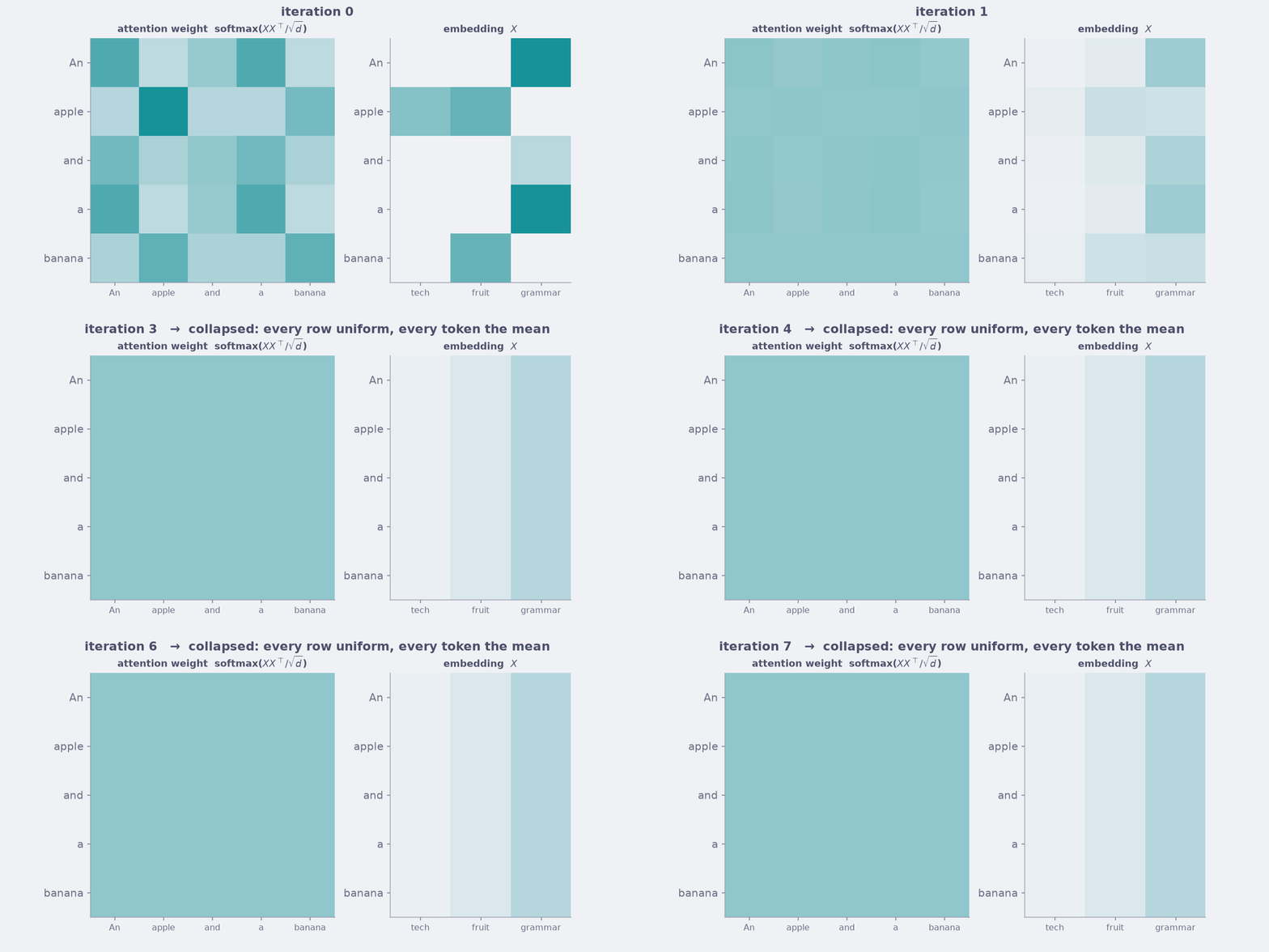
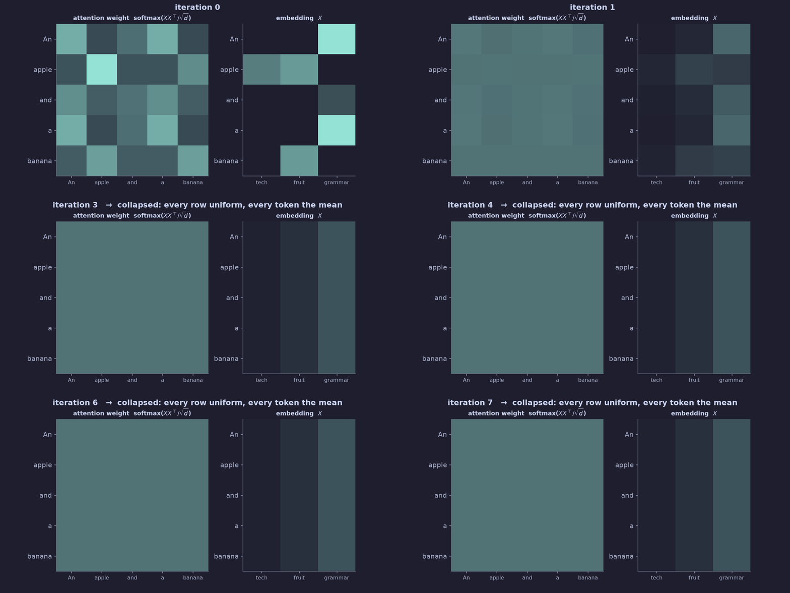
It collapses. By about the fifth iteration every token embedding has converged to the same vector, the batch mean \([0.14, 0.31, 0.52]\), and the attention matrix is a uniform 0.2 in every row. Every token attends equally to every token, which is the same as attending to nothing. The blocky cluster structure from the first pass dissolves into a flat sheet. “an apple and a banana” has become five copies of the average word.
This is representation collapse, and it’s a similar issue we ran into in the JEPA post. Raw self-attention is a smoothing operator, and smoothing without anything to push back eventually erases every distinction.
Splitting the embedding: query, key, value
Raw self-attention has a constraint hiding in it. The embedding of a token is doing two jobs at once. It’s the thing you compare to every other token to decide the weights (the similarity), and it’s the content you average in once the weights are decided (the value). One vector, two jobs, and the model has no freedom to make them different.
Why would you want them different? Because “what am I” and “what do I carry if you pick me” are genuinely different questions. A determiner like “an” is a great signal that a noun follows, so you want other tokens to find it easily, which means its key should advertise “I’m a determiner”. But the content it actually contributes to the average, its value, is thin. It’s grammar, not fruit. With one embedding playing both roles, “an” has to be either findable and content-heavy, or invisible and content-light. It can’t be findable-but-content-light, which is what it actually should be.
The fix is to let the model learn three different linear projections of the embedding, one per role. This is where the query, key, value matrices enter the picture.
- As a query, the projection that says “this is what I’m looking for.”
- As a key, the projection that says “this is what I am.”
- As a value, the projection that says “and this is the content I carry if you pick me.”
Concretely, take the embedding matrix \(X\) and multiply it by three learned weight matrices to get \(Q\), \(K\), \(V\).
\[Q = X W_Q, \quad K = X W_K, \quad V = X W_V\]
The attention weight from \(i\) to \(j\) is now a dot product of \(i\)’s query with \(j\)’s key, because a dot product is still the cheapest possible measure of “do these line up”, but the two sides have been reshaped to whatever the model found useful. Stack all of them into \(Q K^\top\) and the output is that matrix times the values.
\[\text{Attention}(Q, K, V) = \text{softmax}\!\left(\frac{Q K^\top}{\sqrt{d}}\right) V\]
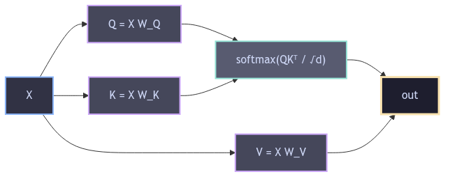
Raw self-attention is the special case where \(W_Q = W_K = W_V = I\), which is exactly what the worked example ran. The code barely changes, the function just takes three arguments instead of one.
function attention(Q, K, V)
    d = size(Q, 2)                    # feature dimension, read off the query
    scores = Q * K' / sqrt(d)        # (n, n) logits
    weights = softmax(scores; dims=2)
    return weights * V               # (n, d)
end
# raw self-attention is the special case attention(X, X, X)
That’s the formula in every textbook, and it’s just a generalisation of \((XX^\top)X\): the three matrices are the model’s freedom to separate “what am I” from “what do I carry”. The raw version is what you get before you give it that freedom.
One head is one kind of question
Single-head attention works, but it has a limitation that’s easy to state and easy to fix. Each query-key pair defines one notion of relevance: “is this token syntactically related”, say, or “is this token in the same entity”. A sentence asks several of those questions at once. “The animal didn’t cross the street because it was too tired” wants “it” to attend to “animal” for coreference, to “street” for a different reading, to “tired” for yet another. One set of weights can only average those demands together, and averaging blunts them.
Multi-head attention is the answer, and the answer is: just run attention several times in parallel with different learned projections, then concatenate.
# h heads, each with its own Q,K,V of dimension d/h, then project back to d
heads = [attention(X * Wq[i], X * Wk[i], X * Wv[i])
        for i in 1:h]
out = hcat(heads...) * Wo
Each head gets a slice of the feature dimension, so the total compute is roughly the same as one full-width head. What you buy with it is specialisation. Different heads learn different relations, and the final projection \(W_O\) lets the model decide how to mix their verdicts. When people visualise attention and show one head tracking verbs and another tracking entities, this is the machinery that makes it possible.
The thing attention cannot do on its own
The attention mechanism I just described is permutation-invariant. If you shuffle the tokens, \(Q\), \(K\), \(V\) get shuffled the same way, the softmax shuffles its rows and columns, and the output is the same shuffle of the same values. Nothing in the attention math knows about order. “The cat sat on the mat” and “mat the on sat cat the” produce the same set of outputs, just reordered.
That’s catastrophic for language, where order carries meaning. So we need to inject position by hand. This can be done by adding a position-dependent vector to each token’s input before any of the projections. Here sines and cosines of different frequencies can do just that.
\[PE_{pos, 2i} = \sin\!\left(\frac{pos}{10000^{2i/d}}\right), \quad PE_{pos, 2i+1} = \cos\!\left(\frac{pos}{10000^{2i/d}}\right)\]
Low-index dimensions oscillate fast (they encode fine position), high-index dimensions oscillate slow (they encode coarse position). Together they give every position a unique fingerprint that’s easy to learn to read off, and because sine and cosine of a related frequency are linear functions of each other, the model can learn simple linear maps for “shift by one position” and “relative offset”, which is what you actually want attention to reason about.
Modern transformers often replace this with learned position embeddings or with rotary position encoding (RoPE), which bakes the rotation directly into the query and key. The principle is the same: attention is order-blind, so you have to put the order in somewhere, and the somewhere is the input.
Stacking, and why it needs help
One layer of attention is a weighted-average machine. To get anything clever, you stack the block. Attention, then a feed-forward network applied to each position, then attention again, and so on, dozens of times. Stacking is where the rest of the architecture shows up, because naive stacking of anything deep is unstable. So how do we fight this instability?
Well, one candidate is the residual connection. Instead of out = layer(x), you write out = x + layer(x). The input is always added back to the output, so the gradient has a direct path back through the stack that doesn’t depend on the layer at all. This is what lets you train networks many layers deep without the gradients vanishing into noise. It comes from ResNet (He et al. 2016), not the transformer paper, but it’s the reason the transformer can be stacked at all.
The second is layer normalisation (Ba et al. 2016). Before (or after, depending on the variant) each sublayer, you normalise the activations across the feature dimension to zero mean and unit variance, then learn a scale and shift. This keeps the activation magnitudes in a sane range across a deep stack, which keeps the softmax and the residual paths well-conditioned.
The original paper does LayerNorm(x + Sublayer(x)) (post-norm); most modern large models do x + Sublayer(LayerNorm(x)) (pre-norm), which trains more stably at depth. The difference is a real engineering choice with measurable effects on training stability, not something to wave away.
The feed-forward block in the middle deserves a word, because it’s easy to dismiss as filler. It’s a two-layer MLP applied independently to each position. Expand the dimension (usually by 4x), apply a nonlinearity, project back down. If attention is the mechanism that mixes information across positions, the feed-forward is the mechanism that processes information within a position. The block alternates the two: mix across, process within, mix across, process within. That alternation is the transformer.
The whole block, in not many lines
Put it together and here’s a single transformer encoder block, in Julia, in about thirty lines. I’m using a pre-norm layout because it’s what I’d actually train:
struct TransformerBlock
    attn_q::Matrix; attn_k::Matrix; attn_v::Matrix; attn_o::Matrix
    ffn_w1::Matrix; ffn_b1::Vector; ffn_w2::Matrix; ffn_b2::Vector
    ln1_scale::Vector; ln1_shift::Vector
    ln2_scale::Vector; ln2_shift::Vector
    n_heads::Int
end

function (b::TransformerBlock)(x)
    # 1. multi-head self-attention, with a residual
    d = size(x, 2); h = b.n_heads; dh = d ÷ h
    xn = layernorm(x, b.ln1_scale, b.ln1_shift)
    Q = xn * b.attn_q; K = xn * b.attn_k; V = xn * b.attn_v
    heads = [attention(Q[:, (i-1)*dh+1:i*dh],
                       K[:, (i-1)*dh+1:i*dh],
                       V[:, (i-1)*dh+1:i*dh])
            for i in 1:h]
    x = x + hcat(heads...) * b.attn_o

    # 2. position-wise feed-forward, with a residual
    xn = layernorm(x, b.ln2_scale, b.ln2_shift)
    x = x + (gelu.(xn * b.ffn_w1 .+ b.ffn_b1)) * b.ffn_w2 .+ b.ffn_b2
    return x
end
That’s it. Stack a few dozen of those, add positional encoding at the bottom, put a language-modelling head on top, and you have a transformer. The block is shown in Figure 2. The paper’s diagram looks intimidating because it shows encoder and decoder and cross-attention, and those matter for translation, but the heart of the thing, the part that’s in every GPT and Llama and Qwen, is the block above.
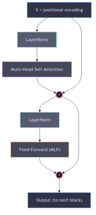
+ nodes are the residual additions; LayerNorm precedes each sublayer; the block alternates multi-head attention (mix across positions) with the feed-forward (process within a position).
The encoder-decoder distinction is worth digging into. The original paper was solving machine translation, so it has two stacks. An encoder that reads the source sentence into rich representations, and a decoder that generates the target one token at a time, attending (via cross-attention) to the encoder’s outputs and (via masked self-attention) to the target tokens generated so far. The causal mask in the decoder is just setting the attention weights for future positions to minus infinity before the softmax, so the model can’t look ahead. Every autoregressive language model, GPT included, is a decoder-only stack with that causal mask baked in. The encoder-only variant (BERT) drops the mask and lets every token see every other token, which is what you want for classification and fill-in-the-blank. Same block, different mask, different training objective.
What I would do next
If I were taking this further, three things.
The first is to actually train the block above on a tiny character-level language model, a few thousand lines of text, and watch the loss come down. I deliberately stopped at the architecture here, because the point was the derivation. But a trained toy is the only proof that the block is wired correctly, and I suspect the exercise would surface the usual small bugs (a transposed weight here, a wrong mask there) that you only find when the loss refuses to drop.
The second is to replace the sinusoidal positional encoding with rotary position encoding (RoPE) (Su et al. 2021).
The third is the residual path and the norm. I’d like to stress-test them. Train the same toy with post-norm vs pre-norm, with and without the residual, with the \(\sqrt{d}\) scaling removed, and just watch. I suspect the ablations would be more instructive than the working version, because they’d show exactly which piece saves which failure mode.
Conclusion
The transformer is one of the most important architectures in modern machine learning, and it is also, as you have seen, a small and reasonable thing. It is a weighted average with learned weights, scaled so the softmax behaves, parallelised across positions, stacked with the help of residuals and normalisation, and given a sense of order by position embeddings pasted on the front.
Why do this? Because, I prefer to understand the thing I’m building on. If you spot a mistake, in the math, in the code, in the intuition, reach out.