price<-function(b, cost, m=1, l=0) (b/(b+1))*((cost-l)/m)As many of us already know R is an extremely useful and powerful language for designing, building and evaluating statistical models. In this example I’m going to use R for calculating the optimal price for a product given very few inputs.
First off we need to define a simple model for the relationship between sales volume (y) and price change (p).
\[ \ln y = \beta \ln p + a \]
The variable a is used as a baseline for our sales. Based on this function we can define a profit function that help us calculate the optimal price based on price elasticity, cost per product produced and profit margin. This function is vectorized and is only defined for price elasticities < -1.0 since that is the condition for finding an optimum. For price elasticities > -1.0 we use a heuristic. In any case the closed formula for the optimal price is given by
\[p=\frac{\beta}{\beta+1}\cdot\frac{c-\lambda}{m}\]
where \(\beta\) is the price elasticity, \(c\) the cost of production, \(m\) the profit margin and \(\lambda\) the penalty term for the case when \(\beta >= -1.0\). In this example \(\lambda\) is set to 0. Price elasticities greater than -1.0 indicates that if the price increases by 1% then the loss in sales is less than 1%. The R code to implement this function is given below.
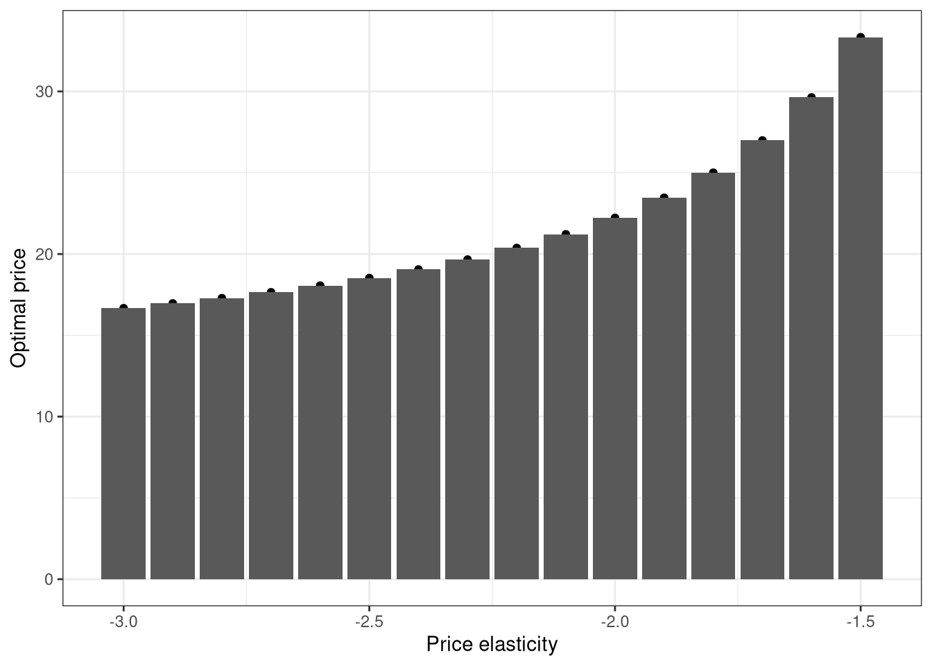
The neat thing about this function is that it’s vectorized by default, which means we can call it using single values or vectors. In the example below we calculate the optimal price based on different price elasticities. We use a fixed cost of 10 and a profit margin of 0.9. Whether or not this is a realistic scenario I will leave up to you to decide. ;)

This small example has shown you how to give quantatative input to the optimal price based on the current price elasticity. Of course the end product would need a more complicated model but the use case is clear and simple. I hope you’ve enjoyed it and will start using R to impress your boss with just how operational it can be.