TL;DR
The COVID-19 virus has struck the world with a rare force (Hui et al. 2020). In a matter of months it has affected 194 countries and territories so far. With respect to Denmark the first confirmed case happened 2020-02-27 and the subject was declared healthy again 2020-03-05 according to Videnskab. In this post we will illustrate the importance of Social distancing in our fight against the Coronavirus. However, we will also dive down into the numbers as to why the model tells us this. Specifically you’ll also learn that the current guidelines of meeting no more than 10 people at a time is really too much. The truth is you should try hard to meet no more than 7 at any given time. And yes, this makes all the difference! So if you’re interested in how we know that social distancing works in epidemics like this read on!
Sweeping declaration: I’m not an epidemiologist, nor do I have any medical training (I’m not that kind of doctor). Thus, I’m in no way qualified to provide domain knowledge of the parameters in the model I will show you. Bear this in mind.
The SEIR model
When dealing with epidemics and infectuous diseases in general where the time from exposure to infection is significant a 4 compartment model called the SEIR (Harko et al. 2014) model is often used. It’s an acronym that stands for Susceptible, Exposed, Infected and Recovered. Susceptible refers to the stock of the population which have the risk on being infected by the disease, i.e., people that are alive and not immune. The Exposed refers to the part of the population that have been infected, but that are not yet showing symptoms. The period from Exposed to Infected is called incubation time. The Infected is exactly what it sounds like; people that have been infected and that are showing symptoms. The last one is Recovered which refers to all subjects that either got a full recovery or died.
The model takes the shape of a Differential Equation since it models how people move between the four compartments. Mathematically we can express the model with these four equations.
\[ \begin{aligned} \frac{dS}{dt} &= (1-S)\mu-\frac{\beta IS}{N}\\ \frac{dE}{dt} &= \frac{\beta IS}{N} - (\sigma+\mu)E\\ \frac{dI}{dt} &= \sigma E - (\gamma+\mu)I\\ \frac{dR}{dt} &= \gamma I - \mu R \end{aligned} \]
The parameters and their interpretation is given in the table below. There are some subleties associated with these parameters but at least this will give you a feel for them.
| Parameter name | Parameter interpretation |
|---|---|
| \(\mu\) | This is the birth rate which is equal to the death rate in this model |
| \(\beta\) | This parameter measures the conversion ratio from susceptible to exposed |
| \(\sigma\) | This parameter governs the incubation period |
| \(\gamma\) | This parameter governs the duration of the infection |
So what are reasobale values for these parameters? Well, to do that we need to use our common sense a bit and do some estimations. But either way it’s all good fun. Now, let’s start with \(\beta\). How can we build an intuition about this? To start with we can realize that only infected people can infect others. So we need to know how effectively they can do that. Basically it will need to consist of at least two factors: (i) the probability \(p\) of actually transferring the virus when they meet another person and (ii) the number of people \(n\) they come into contact with on average each day. Thus we will have \(\beta=pn\) which will make it easier to reason about. Say an average person runs into 20 persons per day and the probability of transferring the virus is 2% we reach a \(\beta=0.02*20=0.4\). Correspondingly, if the chance of transmitting the virus is 4% we end up with \(\beta=0.04*20=0.8\).
For \(\sigma\) we need to think about incubation periods. If the incubation period is around 2–14 days, as we know it is for Covid-19 (Li et al. 2020), we have quite a spread. We can model this incubation period with an exponential distribution \(D\sim\text{Exp}(\sigma)\). This would mean that the average \(E[D]=\frac{1}{\sigma}\) follows from the properties of the Exponential distribution. You can see what the incubation time distribution looks like for \(\sigma=0.25\) in the plot below.
The next parameter we’ll have a look at is the \(\gamma\) which is related to the duration of the infection. Specifically it’s the rate with which infected people recover. We’ll also build an intuition for this using number of days \(L\). Say that an average infection lasts 10 days then an individual recover once every 10 days, if we assume they can be infected again, and this brings us to \(\gamma=1/L\). According to WHO (Organization et al. 2020) it takes between 2 to 8 weeks from symptom onset to recover, for those who died (Yes I know it sounds funny, but recovery in this model refers to death as well as actual recovery). Mild cases typically recover within 14 days. The plot in this case would look like this for a distribution \(L\sim\text{Exp}(\gamma)\)
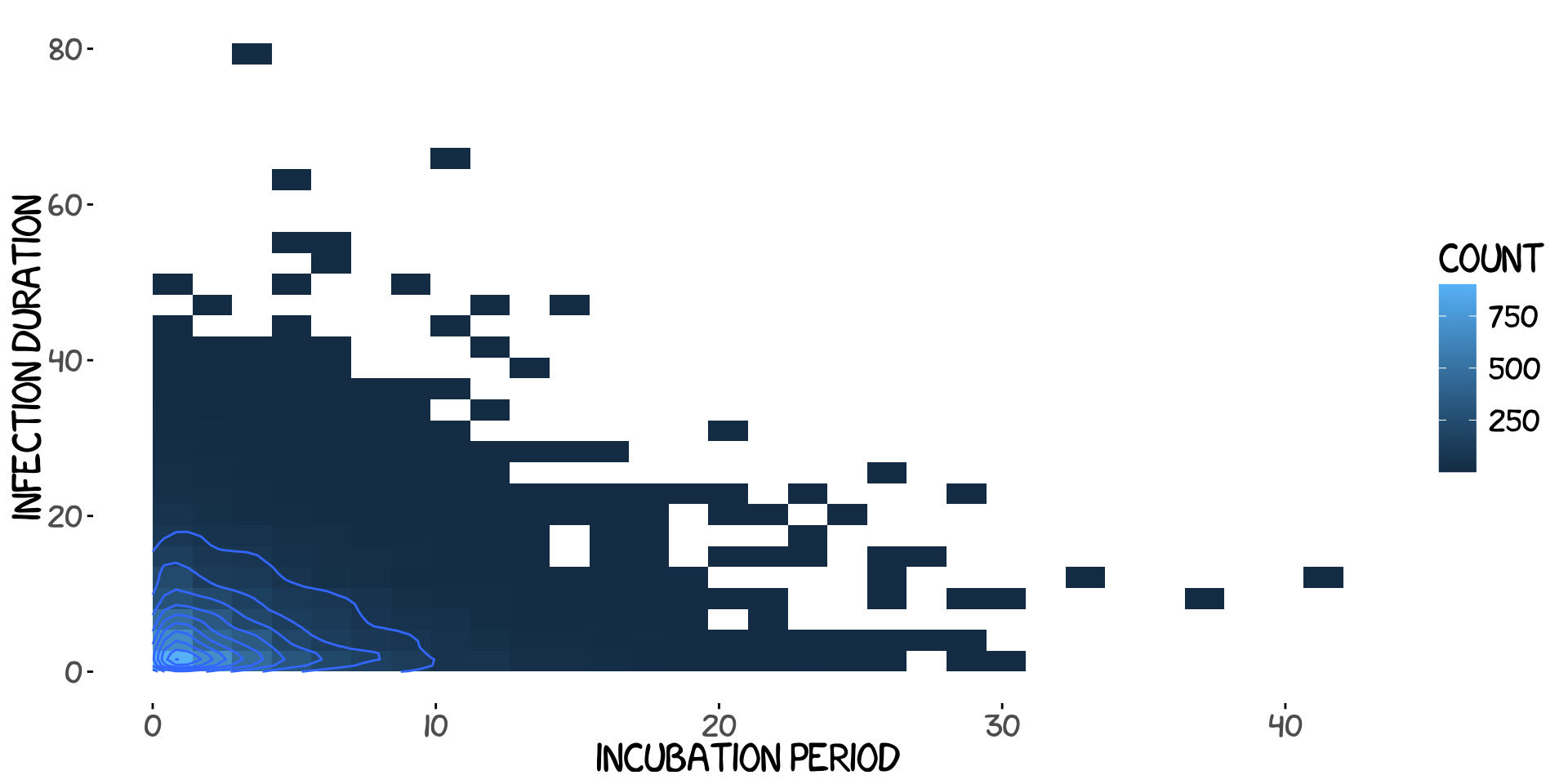
We can look at the joint distribution of \(\sigma\) and \(\gamma\) to see how much longer the infection duration is than the incubation period. We can allow ourselves to do this since we will boldly assume that \(p(\sigma, \gamma)=p(\sigma)p(\gamma)\).
The last parameter of the model is actually the least important and least interesting one, namely the birth rate and death rate. These numbers are given by the Danish Statistical Centre. It’s simply \(\mu=6e4/(5.8e6*365)\) where 365 is needed to put it into daily levels.
So in summary now we have the following parameters to use as a starting point; \(\mu=0.000028, \beta=0.4, \sigma=0.25, \gamma=0.143\) but we’ll play with them more later.
There’s a number that is always quoted when dealing with epidemics and that’s the “Basic Reproduction Number” which measures how many people an infected individual will infect in turn. Mathematically it is given by this relation.
\[R_0 = \frac{\sigma}{\sigma+\mu}\frac{\beta}{\gamma+\mu}\]
As you can see it only uses the parameters of the ODEs which means that we don’t have to solve the equations to get to \(R_0\). In our parameter setting referred to above we would have an \(R_0=2.8\). Just FYI, you really want this number to be below \(1\) or the infection will most likely continue to spread. A bit of algebra will show you that in order to maintain an \(R_0\) below \(1\) you need to keep \(\beta < \gamma\) which means
\[\beta = pn \lt \frac{1}{L}\]
where \(L=7\) is the average number of days an individual stays infected (Velavan and Meyer 2020). This is why you should think twice before meeting a group larger than 7 if \(p\approx 0.02\). If \(p\) instead is around 4% the corresponding maximum number of contacts per day should not exceed 4. We can divide the parameter space of \(\beta\) and \(\gamma\) into a safe \(R_0<1\) and a non-safe \(R_0>1\) area. This is presented in the plot below.
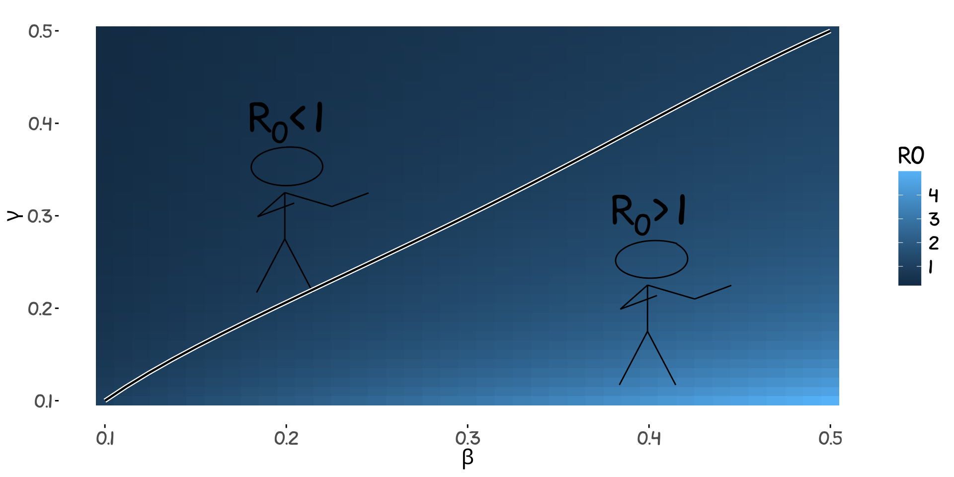
The way to interpret this is:
The longer the infection duration the fewer people we can allow ourselves to meet on a daily basis to keep the infection at bay.
The code
There are many packages around that can create this model and simulations from it but in this post I will show you how to implement it in Julia using just a few lines of code. Basically we need 3 functions. The first function sets up the differential equation of the model. The second one solves the ODEs and then returns an array that we can use for analysis. A quick note here to the observant; You might have noticed that I listed four equations but only define the dynamics of three in the seir_ode function. This is not a bug but a simple usage of the fact that the total population is fixed to \(N=S+E+I+R\) and \(N\) is known since it’s the population of Denmark. This is why \(R\) is given by knowing the others. Thus, seir_ode models the Susceptible \(S\), the Exposed \(E\) and the Infected \(I\), while the seir function adds the \(R\) after the system has been solved.
The last function r0 is calculating the famous “Basic Reproduction Number”.
Anyway, here’s the code given in julia.
using DifferentialEquations

function seir_ode(dY,Y,p,t)
    β, σ, γ, μ = p[1], p[2], p[3], p[4]
    S, E, I = Y[1], Y[2], Y[3]
    dY[1] = μ*(1-S)-β*S*I
    dY[2] = β*S*I-(σ+μ)*E
    dY[3] = σ*E - (γ+μ)*I
end

function seir(β, σ, γ, μ, tspan=(0.0,100.0); S₀=0.99, E₀=0, I₀=0.01, R₀=0)
    par=[β, σ, γ, μ]
    init=[S₀, E₀, I₀]
    seir_prob = ODEProblem(seir_ode,init,tspan,par)
    sol=solve(seir_prob);
    R=ones(1,size(sol)[2])-sum(sol,dims=1);
    hcat(sol.t, sol[1,:], sol[2,:], sol[3,:], R')
end

r0(β, σ, γ, μ) = (σ/(σ+μ))*(β/(γ+μ))
As you might have inferred from the code there is nothing there that does any actual data fitting. We as users need to provide the parameter values to use. In this post we’ll mainly play around with some of the numbers we already know from the Coronavirus spread in the world.
Simulations
We’re going to run two simulations here where we show the importance of social distancing when fighting a disease like the Coronavirus. Each plot will show a vertical bar indicating how far we are today with respect to the progression of the Epidemic. We’re going to keep the other parameters fixed to \(\sigma\approx 0.25\) and \(\gamma \approx 0.15\). Thus in both scenarios \(\beta\) is the only parameter in the model we will vary.
In the first scenario we’re looking at people just going about as they usually do which in our case will mean that you meet around 20 people every day. This is a really bad scenario where we risk having 2 million people infected in Denmark within a couple of months
But what if we limit the number of people we meet and practice the art of Social Distancing? Well then things look a lot better. We can get the maximum number of infected people down by a factor 2. There’s also the benefit of postponing the peak giving the healthcare system time to catch up.
Let’s look at this more specifically with respect to the maximum number of infected people as a consequence of applying the social distancing. Here we say that we can bring the \(\beta\) down from \(0.8\) to \(0.4\). The peak number of projected infected people in Denmark is given by the two rightmost vertical lines for both scenarios.
As you can see we’re talking about a reduction of from 1,682,000 people down to around 928,000.
Now imagine that we could improve that even further? The leftmost vertical line in the plot above shows that we can get the peak down to around 58,000! Say we really change our lives and minimize the amount of contacts. Move all of our social activities to online events and basically stop all traveling. Where do you think we could go with respect to the maximum number of infected people?
The three scenarios discussed is presented in the table below where we have assumed \(p=0.04\) and quantify what that means for the maximum number of people you can meet each day, which day the number of infected people will peak.
| Beta | Contacts | PeakDay | PeakInfected | Scenario |
|---|---|---|---|---|
| 0.3 | 7 | 150 | 58,000 | Successful social distancing |
| 0.4 | 10 | 132 | 928,000 | Partly successful social distancing |
| 0.8 | 20 | 69 | 1,682,000 | Unsuccessful social distancing |
To really put a nail in the coffin with respect to how important social distancing is going to be for our health and economy I would like to show you the progression for the three scenarios in the table above. I’ll also show you where we are today with respect to time.
As you can see we still have time to act, and the time is now. The longer we wait the more difficult it’s going to be to reduce the \(\beta\) and consequently to contain the disease. The question now is, how much are you willing to do to flatten the curve?
Well, that’s all well and good but what about where we are right now. It looks pretty flat and the numbers we’ve seen so far in the news have been much bigger. The numbers in the plot look flat because they are so small in comparison to where the curve is going! Let’s compare the numbers we have registered in Denmark compared to what the model says and fit our parameters based on that. The result is what you can see in the plot below where \(\beta\approx 0.8\), with an incubation time of around 1 day.
We can have a look at this fitted model and predict the progression from it. Now, bear in mind that fitting data this early in a series when dealing with non-linear models is extremely uncertain, but it can serve as a flavor of what might come if we are not careful.
Not so cool, a peak infection affecting 2.32 million people.
Conclusions (what the math tells us)
So no doubt about it math is always fun, but today it’s actually also telling us something of utmost importance for our future way of life. Make no mistake, the Coronavirus is a real thing and the dangers reach far beyond people just getting “the flu”. As we outlined in the beginning of this post we can see that there are two major ways we, as in everyone, can limit the damage of this pandemic.
- Practise social distancing (Keeping the \(n\) low). The rule here is that you should avoid meeting more than around \(7\) people at any time and preferably avoid meeting new people physically right now. The Danish government as of 2020-03-20 recommends meeting less than \(10\) people at any given time, but as we can see that’s not good enough.
- Protect ourselves when meeting people (Keeping the \(p\) low). Here, there are a lot of unknows, but the gist is
- Sneeze in your arm
- Cover your mouth when you cough
- Wear a mask (especially if you have the disease)
- Wash your hands often
- Wipe surfaces you come into contact with often (like your phone)
- Don’t shake hands
- Avoid touching your eyes, nose and mouth
This is something we all can and should do to help fight the pandemic. If we don’t stand together now, it may very well be too late sooner than you think.
References
Harko, Tiberiu, Francisco SN Lobo, and MK Mak. 2014. “Exact Analytical Solutions of the Susceptible-Infected-Recovered (SIR) Epidemic Model and of the SIR Model with Equal Death and Birth Rates.” Applied Mathematics and Computation 236: 184–94.
Hui, David S, Esam I Azhar, Tariq A Madani, et al. 2020. “The Continuing 2019-nCoV Epidemic Threat of Novel Coronaviruses to Global Health—the Latest 2019 Novel Coronavirus Outbreak in Wuhan, China.” International Journal of Infectious Diseases 91: 264–66.
Li, Qun, Xuhua Guan, Peng Wu, et al. 2020. “Early Transmission Dynamics in Wuhan, China, of Novel Coronavirus–Infected Pneumonia.” New England Journal of Medicine.
Organization, World Health et al. 2020. “Report of the Who-China Joint Mission on Coronavirus Disease 2019 (Covid-19).” Available on-Line: Https://Www.who.int/Docs/Default-Source/Coronaviruse/Who-China-Joint-Mission-on-Covid-19-Final-Report.pdf.
Velavan, Thirumalaisamy P, and Christian G Meyer. 2020. “The COVID-19 Epidemic.” Tropical Medicine & International Health.